Introduction to R

R is an interpreted language.

Uses of R

Statistical computations
Predictive analysis
Data visualization by use of libraries e.g. ggplot
Correlation analysis

RULES

Case Sensitivity: R is case sensitive which means functions, variables or object names should be written with the same capitalization. TRUE is different from true.
Comments are added using '#'
Assignment operator:

<- is used instead of =

Rarely uses the right-handed assignment
```
 # Right-handed assignment
 5 -> x
 "Hello" -> message
```
Avoid using reserved keywords as variable names
For variable names use lowercase with words separated by an underscore. Variable names do not have spaces
Do not use zeros to code a factor

Data Types

R supports several data types:

Scalar - A single value with no dimension
Vectors:
- Numeric - stores numbers
- Character - stores texts and strings
- Logical - TRUE/FALSE
Matrices - Two dimensional
Data frames - Two dimensional that can store data of different modes
List - can contain various objects including, vectors, data frames, functions or other lists.

Matrices

All columns in a matrix must have the same mode and same length.

Matrix has to be two dimensional

mymatrix <- matrix(vector, nrow = r, ncol = c, byrow = FALSE,dimnames=list( char_vector_rownames, char_vector_colnames))

byrow=TRUE indicates that the matrix should be filled by rows. byrow=FALSE indicates that the matrix should be filled by columns (the default). dimnames provides optional labels for the columns and rows.

my_matrix[1:3,2:4] results in a matrix with the data on the rows 1, 2, 3 and columns 2, 3, 4.

my_matrix[,1]selects all elements of the first column.

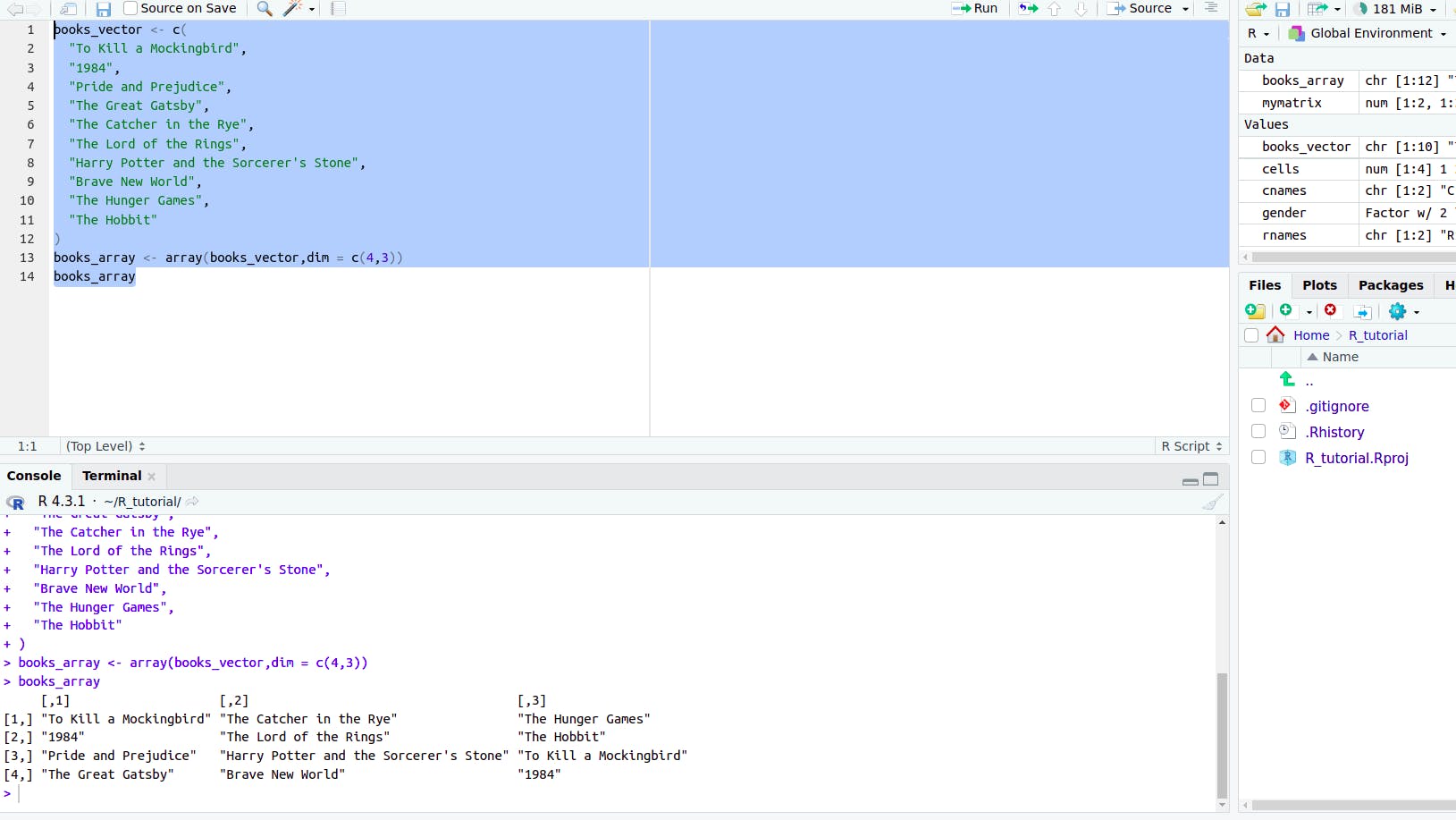
Arrays

Single or multidimensional structure containing data of the same type.

similar to matrices but have more than two dimensions

The dim specifies the dimension of the array sets rows first then columns.

To access an item in the array

Data Frames

Contains correlated information.

They are particularly useful when you need to work with structured data that may have different data types or modes.

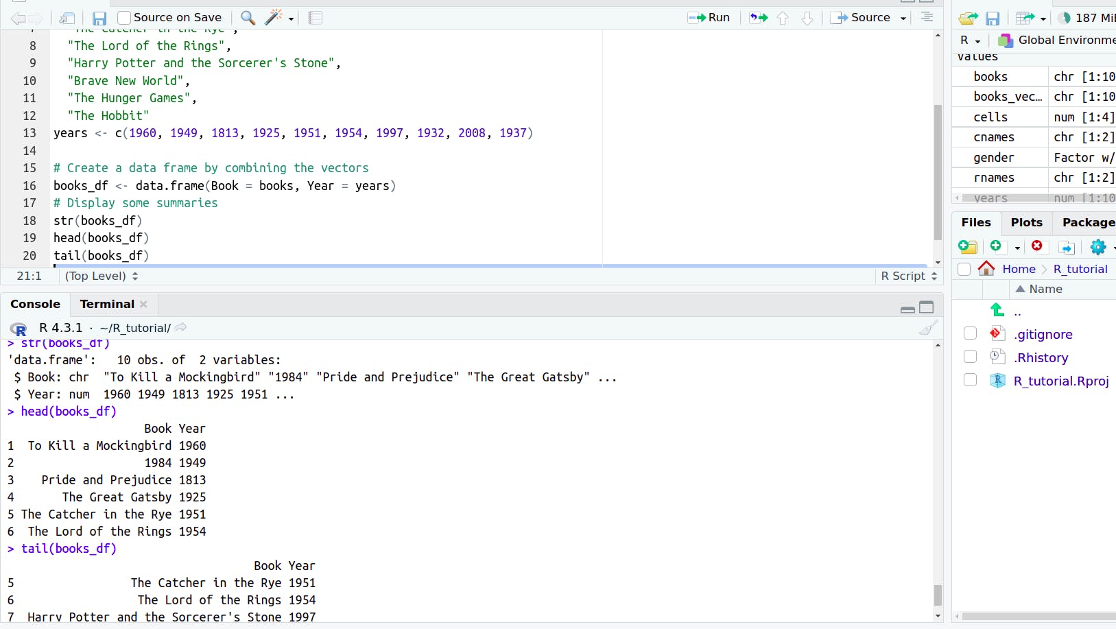
use data.frame() to create a data frame.

characteristics of a data frame

Column names should be nonempty
Row names should be unique
Data stored can be numeric, factor or character types
Each column should contain the same number of data items.

To examine its structure we can use:

str shows the structure

head returns the first 6 elements

tail returns the last 6 elements

nrow displays number of rows(observations)in a data frame

ncol() displays the number of columns (variables) in a data frame

dim()displays the number of rows and columns in a vector of length 2

colnames() display column names

rownames() display the row names

table() creates a frequency table, which displays the counts of unique values or categories in categorical variables.

prop.table() computes proportions. used with the table function.

To manipulate data frames :

rbind() to add rows

cbind() to add columns

To delete an element can use the negative indices

books_df <- books_df[-12,]

Selecting several items from the data frame. T

books_df[1:3,"Year"]

The example will return the first 3 years in the column Year.

Another method is using the column number

books_df[1:3,2]

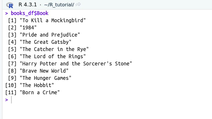
To select an entire column use $

List

An ordered collection of objects.

Allows gathering of unrelated objects under one name.

my_list <- list(comp1, comp2 ...)

Working with lists

Factors

used for representing categorical data with distinct levels or categories

Nominal categorical - no implied order
Ordinal categorical - have orders

gender <- factor(c("Male", "Female", "Male", "Female"))

To view the levels or change the order you can use levels()

factor(some_vector,
       ordered = TRUE,
       levels = c("lev1", "lev2" ...))

ordered : Create an ordered factor.

Vectors

A vector is a basic data structure in R that can store elements of the same data type (e.g., numeric, character, logical).

numeric_vector <- c(1, 2, 3, 4, 5)
character_vector <- c("apple", "banana", "cherry")
logical_vector <- c(TRUE, FALSE, TRUE)

Integer

Whole numbers: positive, zero, negative

Numeric

whole numbers plus numbers with decimal

Character

Text data

working with Vectors

Various operations can be performed on vectors eg arithmetic operations, logical operations and functions for example sum() mean(), length()

Logical

boolean data.

TRUE and FALSE

conversion of data type

as.numeric(): to convert to numeric.

If the original data contains non-numeric it will attempt to convert them to numbers otherwise results in NAs.

# Character vector
character_vector <- c("1", "2", "3", "4", "5")

# Convert to numeric
numeric_vector <- as.numeric(character_vector)

# Print the result
print(numeric_vector)

as.integer(): It rounds down each numeric value to the nearest integer, effectively truncating the decimal part.

If the original data contains non-numeric it will result in an error or produce missing values(NAs).

When applied to logical it converts TRUE to 1 and FALSE to 0

as.character()

# Numeric vector
numeric_vector <- c(1, 2, 3, 4, 5)

# Convert to character
character_vector <- as.character(numeric_vector)

# Print the result
print(character_vector)

as.logical()

# Numeric vector
numeric_vector <- c(0, 1, 0, 1, 0)

# Convert to logical (0 becomes FALSE, 1 becomes TRUE)
logical_vector <- as.logical(numeric_vector)

# Print the result
print(logical_vector)

class() is used to check the data type.